Barotropic-Baroclinic Coupling
Time-averaged accelerations
The barotropic equations are timestepped with a timestep to resolve the surface gravity waves. With care, the baroclinic timestep only need resolve the inertial oscillations. The barotropic accelerations are averaged over the many barotropic timesteps taken between baroclinic steps. At time \(n\), the baroclinic accelerations are computed. The vertical average of that acceleration is subtracted off and replaced by the time-averaged acceleration from the group of barotropic timesteps:
Similarly, the velocities used in the tracer equation are a careful blend of the barotropic and baroclinic solutions:
with
Two estimates of the free surface height
The vertically discrete, temporally continuous layer continuity equations are:
The relationship between the free surface height and the layer thicknesses \(h_k\) is:
We get an evolution equation for the free surface height:
If the algorithms for the fluxes in the continuity equations are linear in the velocity, the free surface height can be rewritten as:
where
However, ALE models like MOM6 require positive-definite, nonlinear continuity solvers (MOM6 uses PPM Advection Scheme). We need a different way to reconcile this estimate of free surface height with the one coming from the barotropic equations. After rejecting several other options, MOM6 is now using the scheme from [39]. The barotropic update of \(\eta\) is given by:
Determine the \(\Delta U\) such that:
where
The layer timestep equation becomes:
This scheme has these properties:
Total mass is conserved layer-wise.
Layer equations retain their flux form.
Total salt, heat, and other tracers are exactly conserved.
Free surface heights exactly agree.
Requires (very few) completely local iterations.
The velocity corrections are barotropic, and more likely to correspond to the layers whose flow was deficient than in some older schemes.
The solution is unique provided that:
This is a reasonable requirement for any discretization of the continuity equation. In the continuous limit, \(\mathbf{F} (u,h) = uh\), so one interpretation is:
With the PPM continuity scheme:
leads to:
\(h_i(x) > 0\) is already required for positive definiteness.
Newton’s method iterations quickly give \(\Delta U\):
How practical is this iterative approach?
The piecewise parabolic method continuity solver uses two steps:
Set up the positive-definite subgridscale profiles, \(h_{PPM}(x)\).
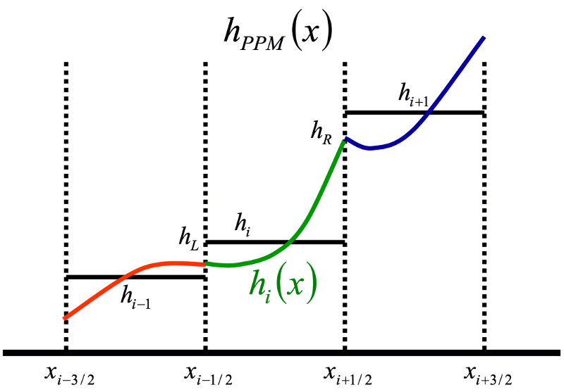
Piecewise parabolic reconstructions of \(h(x)\).
Integrating the profiles to determine \(F\). Step 1 is typically \(\sim 3\) times as expensive as step 2. \(F(u,h)\) is piecewise cubic in \(u\), but often nearly linear. Newton’s method iterations converge quickly:
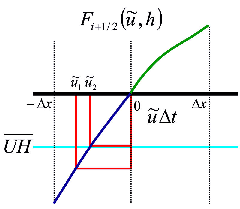
Newton’s method iterations for finding \(\Delta U\).
In a global model the sea surface heights converge everywhere to a tolerance of \(10^{-6}\) m within five iterations. These five iterations add \(\sim 1.6\) times more CPU time to the PPM continuity solver and the continuity solver is just 12% of the total model time.
A note on bottom drag
Barotropic accelerations do not lead to barotropic flows after a timestep when vertical viscosity is taken into account.
A tridiagonal equation for \(\gamma_k\) results, going from 0 for thin layers near the bottom to 1 far above the bottom.
In the continuous limit:
with boundary conditions:
For deep water and constant \(\nu\), we get:
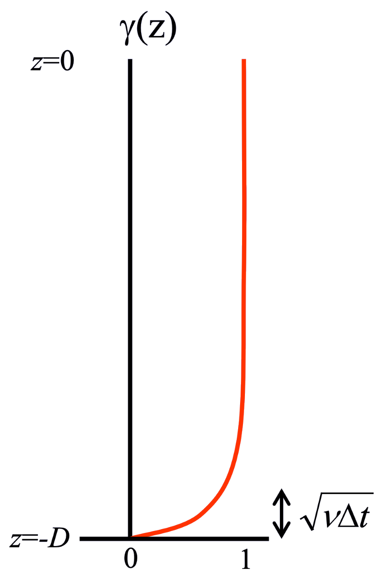
The continuous solution for barotropic flow plus a no-slip condition at the bottom.
We want a scheme in which the split model looks exactly like the unsplit model would if we had taken all those short 3D timesteps. Rather than applying a barotropic velocity, we use a barotropic acceleration and allow the continuity solver to determine the transports consistent with a no-slip bottom boundary layer and perhaps also a no-slip surface boundary layer under an ice shelf.
From above, the barotropic equation is:
We need to determine the \(\Delta \overline{A}\) such that:
where
Additional details about the split time stepping
Transports are used as input and output to the barotropic solver. The continuity solver is inverted to determine velocities.
We need to find \(\Delta \overline{u}\) such that:
Barotropic accelerations are treated as anomalies from the baroclinic state:
Bottom drag (and under ice surface-drag) is treated implicitly.
The barotropic continuity solver uses flow-dependent thickness fits which approximate the sum of the layer thickness transports, to accommodate wetting and drying. An image of this is shown here:
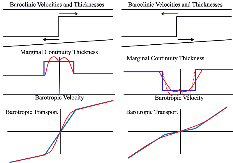
The barotropic transports depend on the baroclinic flows and thicknesses.
Summary of MOM6 split time stepping
We use an efficient approach for handling fast modes via simplified 2-d equations, while the 3-d baroclinic timestep is determined by baroclinic dynamics.
The barotropic solver determines free surface height and time-averaged depth-integrated transports.
By using anomalies, the MOM6 split solver gives identical answers to an equivalent unsplit scheme for short timesteps.
This scheme has been demonstrated to work with wetting and drying, as well as under ice-shelves.
The linear barotropic solver allows MOM6 to automatically set a stable barotropic timestep (e.g. to 98% of maximum).