PPM Advection Scheme

Advection Scheme

Following [11] and [10], we use the Piecewise Parabolic Method (PPM) to represent values within the model cells. Each cell is assumed to have a piecewise parabolic representation, which is uniquely prescribed by conservation and the two edge values. This method has the following features:

• The PPM approach is conservative.

• The (unlimited) order of accuracy is determined by the estimates of the edge values.

• Monotonicity is ensured by adjusting the edge values to flatten the profile.

An example is shown in this figure:

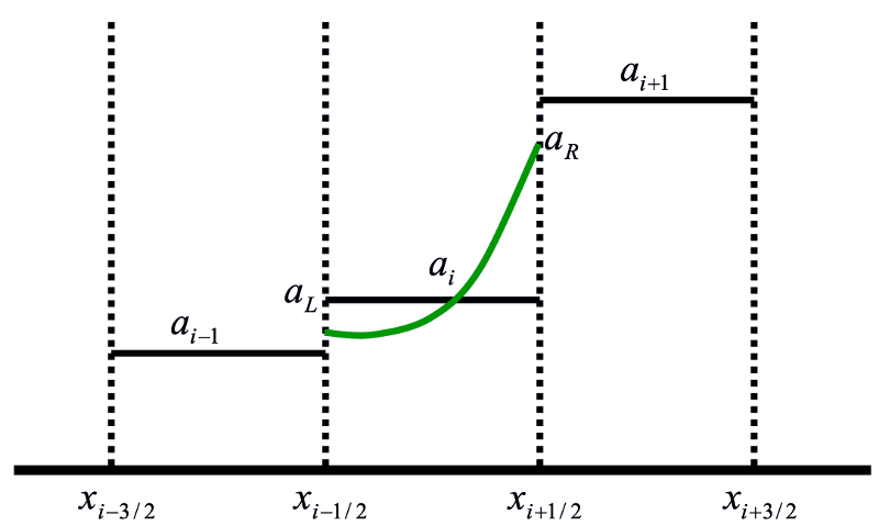
The parabolic representation of a field within a cell.

\[x'_i \equiv \frac{x - x_{i-1/2}} {\Delta x_i}\]

\[\Delta x_i \equiv x_{i + 1/2} - x_{i- 1/2}\]

\[c \equiv u \Delta t / \Delta x_i\]

\[A_i(x') = a_L + (a_R - a_L) x'_i + a_6 x'_i(1 - x'_i)\]

\[a_6 = 6a_i - 3 (a_R + a_L)\]

\[\begin{split}\begin{eqnarray} a_i &= \int_0^1 A_i(x'_i) dx'_i = \int_0^1 a_L + (a_R - a_L) x'_i + a_6 x'_i (1 - x'_i) dx'_i \\ &= \left[ a_L x'_i + \frac{1}{2} (a_R - a_L) x_i^{\prime 2} + a_6 \left( \frac{1}{2} x_i^{\prime 2} - \frac{1}{3} x_i^{\prime 3} \right) \right]_0^1 \\ &= \frac{1}{2} (a_R + a_L) + \frac{1}{6} a_6 \end{eqnarray}\end{split}\]

\[\begin{split}\begin{eqnarray} F_{i+1/2} &= \frac{1}{\Delta t} \int_{x_{i + 1/2} - u \Delta t}^{x_{i + 1/2}} A_i^n(x) dx = \frac{\Delta x}{\Delta t} \int_{1-c}^1 A_i (x'_i) dx'_i \\ &= \frac{\Delta x}{\Delta t} \left[ a_L x'_i + \frac{1}{2} (a_R - a_L) x_i^{\prime 2} + a_6 \left( \frac{1}{2} x_i^{\prime 2} - \frac{1}{3} x_i^{\prime 3} \right) \right]_{1 - c}^1 \\ &= \frac{\Delta x}{\Delta t} \left[ a_L c + (a_R - a_L + a_6) \left( c - \frac{1}{2} c^2 \right) - a_6 \left( c - c^2 + \frac{1}{3} c^3 \right) \right] \\ &= u \left[ a_R + \frac{1}{2} (a_L - a_R) c + a_6 \left( \frac{1}{2} c - \frac{1}{3} c^2 \right) \right] \end{eqnarray}\end{split}\]

The choice of \(a_L\) and \(a_R\) is not unique, but can be done according to [11] (CW84) or [34] (H3) as mentioned in Tracer Advection.