Horizontal indexing and memory
Conventions for staggering of variables and loops over 2d/3d arrays
MOM6 is written in Fortran90 and uses the i,j,k order of indexing. i corresponds to the fastest index (stride-1 in memory) and thus should be the inner-most loop variable. We often refer to the i-direction as the x- or zonal direction, and similarly to the j-direction as y- or meridional direction. The model can use curvilinear grids/coordinates in the horizontal and so these labels have loose meanings but convenient.
Loops and staggered variables
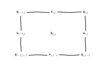
Many variables are staggered horizontally with respect to each other. The dynamics and tracer equations are discretized on an Arakawa C grid. Staggered variables must still have integer indices and we use a north-east convention centered on the h-points. These means a variable with indices i,j will be either collocated, to the east, to the north, or to the north-east of the h-point with the same indices.

MOM6 uses an Arakawa C grid staggering of variables with a North-East indexing convention. “Cells” refer to the control volumes around tracer- or h-point located variables unless labelled otherwise.
Soft convention for loop variables
To ease reading the code we use a “soft” convection (soft because there is no syntax checking) where an upper-case index variable can be interpreted as the lower-case index variable plus \(\frac{1}{2}\).
For example, when a loop is over h-points collocated variables
* the do-loop statements will be for lower-case i,j variables
references to h-point variables will be
h(i,j),D(i+1,j), etc.references to u-point variables will be
u(I,j)(meaning \(u_{i+\frac{1}{2},j}\)),u(I-1,j)(meaning \(u_{i-\frac{1}{2},j}\)), etc.references to v-point variables will be
v(i,J)(meaning \(v_{i,j+\frac{1}{2}}\)),u(I-1,j)(meaning \(u_{i,j-\frac{1}{2}}\)), etc.references to q-point variables will be
q(I,J)(meaning \(q_{i+\frac{1}{2},j+\frac{1}{2}}\)), etc.
In contrast, when a loop is over u-points collocated variables
* the do-loop statements will be for upper-case I and lower-case j variables
the expression \(u_{i+\frac{1}{2},j} ( h_{i,j} + h_{i+1,j} )\) is
u(I,j) * ( h(i,j) + h(i+1,j).
Declaration of variables

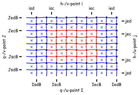
Non-symmetric mode: All arrays are declared with the same shape (isd:ied,jsd:jed).

Symmetric mode: Arrays have different shapes depending on their staggering location on the Arakawa C grid.
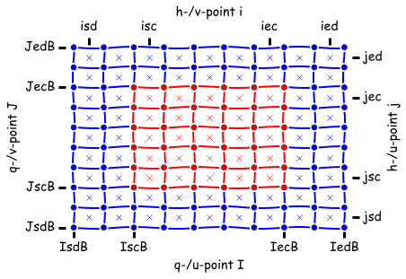
A field is described by 2D or 3D arrays which are distributed across parallel processors. Each processor only sees a small window of the global field. The processor “owns” the computational domain (red in above figure) but arrays are extended horizontally with halos which are intermittently updated with the values from neighboring processors. The halo regions (blue in above figure) may not always be up-to-date. Data in halo regions (blue in above figure) will be overwritten my mpp_updates.
MOM6 has two memory models, “symmetric” and “non-symmetric”. In non-symmetric mode all arrays are given the same shape. The consequence of this is that there are fewer staggered variables to the south-west of the computational domain. An operator applied at h-point locations involving u- or v- point data can not have as wide a stencil on the south-west side of the processor domain as it can on the north-east side.
In symmetric mode, declarations are dependent on the variables staggered location on the Arakawa C grid. This allows loops to be symmetric and stencils to be applied more uniformly.
In the code, declarations are consistent with the symmetric memory model. The non-symmetric mode is implemented by setting the start values of the staggered data domain to be the same as the non-staggered start value.
The horizontal index type (mom_hor_index::hor_index_type()) provides the data domain start values. The values are also copied into the ) provides the data domain start values. The values are also copied into the mom_grid::ocean_grid_type() for convenience although we might deprecate this convenience in the future.for convenience although we might deprecate this convenience in the future.
Declarations of h-point data take the form:
* real, dimension(HI%isd:HI%ied, HI%jsd:HI%jed) :: D !< Depth at h-points (m)
real, dimension(HI%isd:HI%ied, HI%jsd:HI%jed, GV%ke) :: h !< Layer thickness (H units)
Declarations of u-point data take the form:
* real, dimension(HI%IsdB:HI%IedB, HI%jsd:HI%jed) :: Du !< Depth at u-points (m)
real, dimension(HI%IsdB:HI%IedB, HI%jsd:HI%jed, GV%ke) :: h !< Zonal flow (m/s)
Declarations of v-point data take the form:
* real, dimension(HI%isd:HI%ied, HI%JsdB:HI%JedB) :: Dv !< Depth at v-points (m)
real, dimension(HI%isd:HI%ied, HI%JsdB:HI%JedB, GV%ke) :: h !< Zonal flow (m/s)
Declarations of q-point data take the form:
* real, dimension(HI%IsdB:HI%IedB, HI%JsdB:HI%JedB) :: Dq !< Depth at q-points (m)
real, dimension(HI%IsdB:HI%IedB, HI%JsdB:HI%JedB, GV%ke) :: vort !< Vertical componentof vorticity (s-1)
The file MOM_memory_macros.h provides the macros SZI_, SZJ_, SZIB_ and SZJB_ that help make the above more concise:
* real, dimension( SZI_(HI) , SZJ_(HI) ) :: D !< Depth at h-points (m)
real, dimension( SZIB_(HI) , SZJ_(HI) ) :: Du !< Depth at u-points (m)real, dimension( SZI_(HI) , SZJB_(HI) ) :: Dv !< Depth at v-points (m)real, dimension( SZIB_(HI) , SZJB_(HI) ) :: Dq !< Depth at q-points (m)
See MOM_memory_macros.h for the complete list of macros used in various memory modes.
Calculating a global index
For the most part MOM6 code should be independent of an equivalent absolute global index. There are exceptions and when the global index of a cell i,j is needed is can be calculated as follows:
i_global = i + HI%idg_offset
Before the mom_hor_index::hor_index_type() was introduced, this conversion was done use variables in the was introduced, this conversion was done use variables in the mom_grid::ocean_grid_type()::
i_global = (i-G%isd) + G%isd_global
which is no longer preferred.
Note that a global index only makes sense for a rectangular global domain. If the domain is a Mosaic of connected tiles (e.g. size tiles of a cube) the global indices (i,j) become meaningless.