Vertical Lagrangian method: conceptual

Lagrangian and ALE

As discussed by Adcroft and Hallberg (2008) [2] and Griffies, Adcroft and Hallberg (2020) [22], we can conceive of two general classes of algorithms that frame how hydrostatic ocean models are formulated. The two classes differ in how they treat the vertical direction. Quasi-Eulerian methods follow the approach traditionally used in geopotential coordinate models, whereby vertical motion is diagnosed via the continuity equation. Quasi-Lagrangian methods are traditionally used by layered isopycnal models, with the vertical Lagrangian approach specifying motion that crosses coordinate surfaces. Indeed, such dia-surface flow can be set to zero using Lagrangian methods for studies of adiabatic dynamics. MOM6 makes use of the vertical Lagrangian remap method, as pioneered for ocean modeling by Bleck (2002) [7] and further documented by [22], with this method a limit case of the Arbitrary-Lagrangian-Eulerian method ([33]). Dia-surface transport is implemented via a remapping so that the method can be summarized as the Lagrangian plus remap approach and so it is a one-dimensional version of the incremental remapping of Dukowicz (2000) [13].

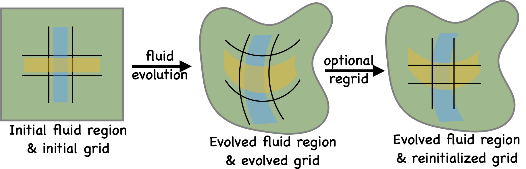
Schematic of the 3d Lagrangian regrid/remap method

Refer to the above figure taken from Griffies, Adcroft, and Hallberg (2020) [22]. It shows a schematic of the Lagrangian-remap method as well as the Arbitrary Lagrangian-Eulerian (ALE) method. The first panel shows a square fluid region and square grid used to represent the fluid, along with rectangular subregions partitioned by grid lines. The second panel shows the result of evolving the fluid region and evolving the grid. The grid can evolve according to the fluid flow, as per a Lagrangian method, or it can evolve according to some specified grid evolution, as per an ALE method. The right panel depicts the grid reinitialization onto a target grid (the regrid step). A regrid step necessitates a corresponding remap step to estimate the ocean state on the target grid, with conservative remapping required to preserve integrated scalar contents (e.g., potential enthalpy, salt mass, and seawater mass). The regrid/remap steps are needed for Lagrangian methods in order for the grid to retain an accurate representation of the ocean state. Ideally, the remap step does not affect any changes to the fluid state; rather, it only modifies where in space the fluid state is represented. However, any numerical realization incurs interpolation inaccuracies that lead to unphysical (spurious) state changes.

Vertical Lagrangian regrid/remap method

We now get a bit more specific to the vertical Lagrangian method. For this purpose, recall recall the basic dynamical equations (those equations with a time derivative) of MOM6 discussed in Generalized vertical coordinate equations

(5)\[\begin{split}\begin{align} \rho_0 \left[ \frac{\partial \mathbf{u}}{\partial t} + \frac{( f + \zeta )}{h} \, \hat{\mathbf{z}} \times h \, \mathbf{u} + \underbrace{ \dot{r} \, \frac{\partial \mathbf{u}}{\partial r} } \right] &= -\nabla_r \, (p + \rho_{0} \, K) - \rho \nabla_r \, \Phi + \mathbf{\mathcal{F}} &\mbox{horizontal momentum} \label{eq:h-horz-momentum-vlm} \\ \frac{\partial h}{\partial t} + \nabla_r \cdot \left( h \, \mathbf{u} \right) + \underbrace{ \delta_r ( z_r \dot{r} ) } &= 0 &\mbox{thickness} \label{eq:h-thickness-equation-vlm} \\ \frac{\partial ( \theta \, h )}{\partial t} + \nabla_r \cdot \left( \theta h \, \mathbf{u} \right) + \underbrace{ \delta_r ( \theta \, z_r \dot{r} ) } &= h \mathbf{\mathcal{N}}_\theta^\gamma - \delta_r J_\theta^{(z)} &\mbox{potential/Conservative temp} \label{eq:h-temperature-equation-vlm} \\ \frac{\partial ( S \, h )}{\partial t} + \nabla_r \cdot \left( S \, h \, \mathbf{u} \right) + \underbrace{ \delta_r ( S \, z_r \dot{r} ) } &= h \mathbf{\mathcal{N}}_S^\gamma - \delta_r J_S^{(z)} &\mbox{salinity} \label{eq:h-salinity-equation-vlm} \end{align}\end{split}\]

The MOM6 implementation of the vertical Lagrangian method makes use of two general steps. The first evolves the ocean state forward in time according to a vertical Lagrangian approach with with \(\dot{r}=0\). Hence, the horizontal momentum, thickness, and tracers are time stepped with the underbraced terms removed in the above equations. All advective transport occurs within a layer as defined by constant \(r\)-surfaces so that the volume within each layer is fixed. All other terms are retained in their full form, including subgrid scale terms that contribute to the transfer of tracer and momentum into distinct \(r\) layers (e.g., dia-surface diffusion of tracer and velocity). Maintaining constant volume within a layer yet allowing for tracers to move between layers engenders no inconsistency between tracer and thickness evolution. The reason is that tracer diffusion, even dia-surface diffusion, does not transfer volume.

The second step in the method comprises the generation of a new vertical grid following a prescription, such as whether the grid should align with isopcynals or constant \(z^{*}\) or a combination. This second step is known as the regrid step. The ocean state is then vertically remapped to the newly generated vertical grid. This remapping step incorporates dia-surface transfer of properties, with such transfer depending on the prescription given for the vertical grid generation. To minimize discretization errors and the associated spurious mixing, the remapping step makes use of the high order accurate methods developed by [68] and [69].

Outlining the numerical algorithm

The underlying algorithm for treatment of the vertical can be related to operator-splitting of the underbraced terms in the above equations. If we consider, for simplicity, an Euler-forward update for a time-step \(\Delta t\), the time-stepping for the thickness and tracer equation ( \(C\) is an arbitrary tracer) can be summarized as (from Table 1 in Griffies, Adcroft and Hallberg (2020) [22])

(6)\[\begin{split}\begin{align} \delta_{r} w^{\scriptstyle{\mathrm{grid}}} &= -\nabla_{r} \cdot [h \, \mathbf{u}]^{(n)} &\mbox{layer motion via horz conv} \\ h^{\dagger} &= h^{(n)} + \Delta t \, \delta_{r} w^{\scriptstyle{\mathrm{grid}}} = h^{(n)} - \Delta t \, \nabla_{r} \cdot [h \, \mathbf{u}]^{(n)} &\mbox{update thickness via horz advect} \\ [h \, C]^{\dagger} &= [h \, C]^{(n)} -\Delta t \, \nabla_{r} \cdot [ h \, C \, \mathbf{u} ]^{(n)} &\mbox{update tracer via horz advect} \\ h^{(n+1)} &= h^{\scriptstyle{\mathrm{target}}} &\mbox{regrid to the target grid} \\ \delta_{r} w^{(\dot{r})} &= -(h^{\scriptstyle{\mathrm{target}}} - h^{\dagger})/\Delta t &\mbox{diagnose dia-surface transport} \\ [h \, C]^{(n+1)} &= [h \, C]^{\dagger} - \Delta t \, \delta_{r} ( w^{(\dot{r})} \, C^{\dagger}) &\mbox{remap tracer via dia-surface transport} \end{align}\end{split}\]

The first three equations constitute the Lagrangian portion of the algorithm. In particular, the second equation provides an intermediate or predictor value for the updated thickness, \(h^{\dagger}\), resulting from the vertical Lagrangian update. Similarly, the third equation performs a Lagrangian update of the thickness-weighted tracer to intermediate values, again operationally realized by dropping the \(w^{(\dot{r})}\) contribution. The fourth equation is the regrid step, which is the key step in the algorithm with the new grid defined by the new thickness \(h^{(n+1)}\). The new thickness is prescribed by the target values for the vertical grid,

\[\begin{align} h^{(n+1)} = h^{\scriptstyle{\mathrm{target}}}. \end{align}\]

The prescribed target grid thicknesses are then used to diagnose the dia-surface velocity according to

\[\begin{align} \delta_{r} w^{(\dot{r})} = -(h^{\scriptstyle{\mathrm{target}}} - h^{\dagger})/\Delta t. \end{align}\]

This step, and the remaining step for tracers, constitute the remapping portion of the algorithm. For example, if the prescribed coordinate surfaces are geopotentials, then \(w^{(\dot{r})}\) and \(h^{\scriptstyle{\mathrm{target}}} = h^{(n)}\), in which case the remap step reduces to Cartesian vertical advection.

Within the above framework for evolving the ocean state, we make use of a standard split-explicit time stepping method by decomposing the horizontal momentum equation into its fast (depth integrated) and slow (deviation from depth integrated) components. Furthermore, we follow the methods of Hallberg and Adcroft (2009) [30] to ensure that the free surface resulting from time stepping the depth integrated thickness equation (i.e., the free surface equation) is consistent with the sum of the thicknesses that result from time stepping the layer thickness equations for each of the discretized layers; i.e., \(\sum_{k} h = H + \eta\).